Azure ML Pipelines and MLOps with GitHub Actions – Part 3

As this is Part 3, you might want to review Part 1 and Part 2 for context if you haven’t yet.

In Part 3, I will finally focus on the GitHub action.

All of the code for this can be found on my GitHub.

How to run the training process from GitHub Action

To put the "Ops" in "MLOps" the pipeline execution should be automated whenever possible. The scenario being used in this repository is when code is checked in, the training pipeline is automatically kicked off from a GitHub Action and if the newly trained model has a higher accuracy than the previous model, then it will be registered in the model repository.

To review, iris_supervised_model.py does the training and register_model.py obviously registers the model. The pipeline that runs these two steps is built and executed from train_pipeline.py. So it is this train_pipeline.py (also referred to in this repository documentation as the driver script) that needs to be executed from a GitHub action.

Creating the GitHub Action

Actions allow for automation of processes. They are YAML scripts.

I won’t pretend to be an expert on YAML or the action schema, but i pulled a sample and made some modifications. Action scripts should be placed in .github/workflows directory of the repo.

name: iristrain
on: [push]
jobs:
  run:
    runs-on: [ubuntu-latest]
    container: docker://dvcorg/cml-py3:latest
    steps:
      - uses: actions/checkout@v2
      - name: train_pipeline
        env:
          repo_token: ${{ secrets.GITHUB_TOKEN }}
          AZUREML_CLIENTID: ${{secrets.AZUREML_CLIENTID}}
          AZUREML_TENANTID: ${{secrets.AZUREML_TENANTID}}
          AZUREML_SECRET: ${{secrets.AZUREML_SECRET}}
          AZUREML_SUBSCRIPTION: ${{secrets.AZUREML_SUBSCRIPTION}}
          AZUREML_RESOURCE_GROUP: ${{secrets.AZUREML_RESOURCE_GROUP}}
          AZUREML_WORKSPACE: ${{secrets.AZUREML_WORKSPACE}}
        run: |
          # Your ML workflow goes here
          pip install -r requirements.txt
          python azureml/train_pipeline.py

The above code shows that on [push] so when any code is pushed to the repository, the jobs: will be performed. Unique to this example is the environment variables env: that are all populated from GitHub secrets. They are passed into the train_pipeline.py script which is invoked with the last line of the yaml file above. Any libraries required to run the python script need to be installed first on the container therefore the pip install -r requirements.txt is there. The current requirements.txt has more than what is needed to run the script, specifically azureml-sdk is the entry required for this scenario.

Service Principal Authentication to Azure ML

Unlike building a pipeline and running it from a Jupyter notebook interactively, to use automation the credentials to login to Azure ML have to be stored. Using an Azure Active Directory user principal is the right way to do this.

Creating a service principal in Azure will likely require elevated permissions in Azure. Work with your Azure administrator to enable this.

In this notebook there is a section for Service Principal Authentication that walks through the setup. Once a service principal is created, it can be used from the train_pipeline.py script.

from azureml.core import Workspace
from azureml.core.authentication import ServicePrincipalAuthentication

svc_pr_password = os.environ.get("AZUREML_SECRET")
svc_pr = ServicePrincipalAuthentication(
    tenant_id=os.environ['AZUREML_TENANTID'],
    service_principal_id=os.environ['AZUREML_CLIENTID'],
    service_principal_password=svc_pr_password)

ws = Workspace(
    subscription_id=os.environ['AZUREML_SUBSCRIPTION'],
    resource_group=os.environ['AZUREML_RESOURCE_GROUP'],
    workspace_name=os.environ['AZUREML_WORKSPACE'],
    auth=svc_pr
    )

Note the heavy use of environment variables. This is to ensure that credentials and other private variables are not stored clear text in this repo for the world to see. These are being passed in from the action yaml shown above.

More comprehensive information on Azure ML authentication can be found here

GitHub Secrets

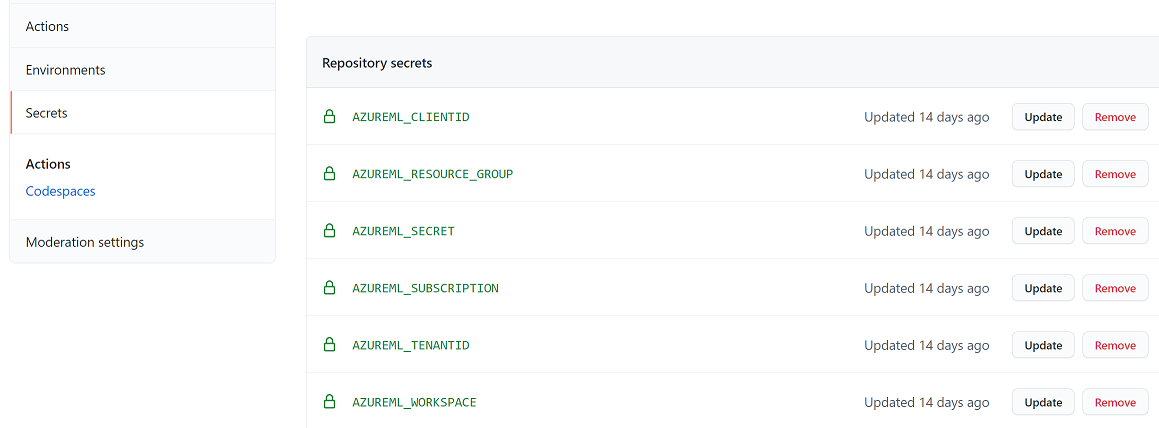
The above section highlights the environment variables being used. These variables are initiated from the GitHub repositories action secrets.

GitHub Secrets

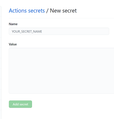
These secrets are created in the repository from the "Settings" tab. In the "Secrets" section, click the "new repository secret" button to add a secret.

GitHub New Secret

It should be obvious that the secret names need to match the secrets given in the yaml action script: ${{secrets.AZUREML_CLIENTID}}.

Invoking the GitHub Action

Any change to the source code based on this simple action definition will invoke the train_pipeline.py which defines and then submits the iris_train_pipeline with the snip of code below.

iris_train_pipeline = Pipeline(workspace=ws, steps=[trainingScript,registerModelStep])
print ("Pipeline is built")

exp = Experiment(ws,experiment_name)
exp.set_tags({'automl':'no','working':'no'})

pipeline_run1 = exp.submit(iris_train_pipeline)
print("Pipeline is submitted for execution")

pipeline_run1.wait_for_completion()

This will happen from master or a branch. To see the action in action, in iris_supervised_model.py change the n_splits from 5 to 3.

code change example

Do a commit and push. Note: I have been using VSCode. The Python editor and GitHub integration is legit!

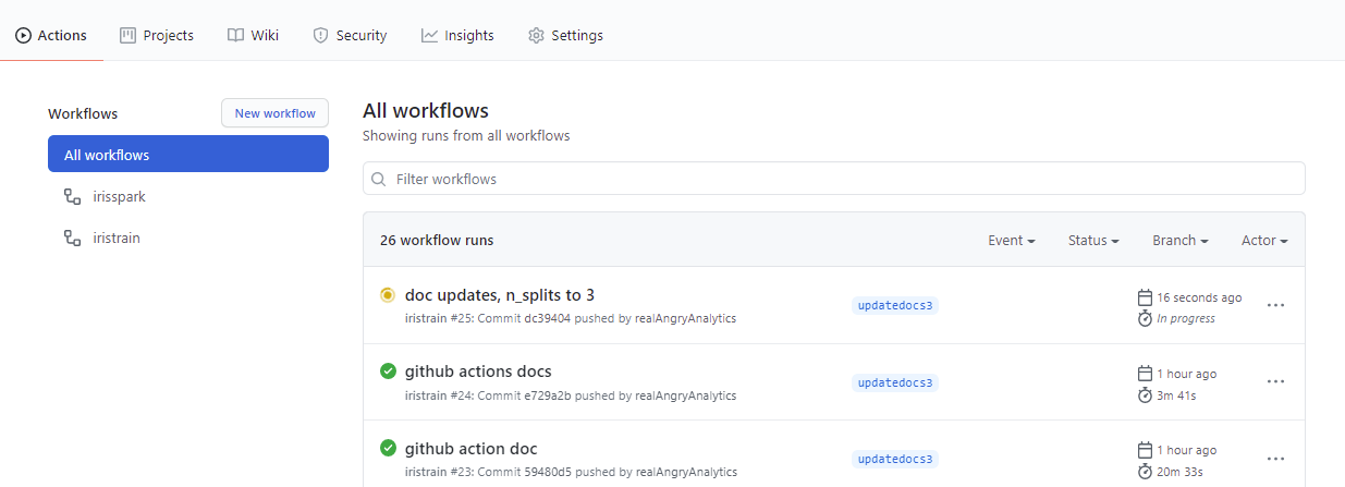
On the Actions tab of the repo, a new action is now visible with a "yellow" icon to indicate "in progress" actions list

Click on the run to see the details in progress action

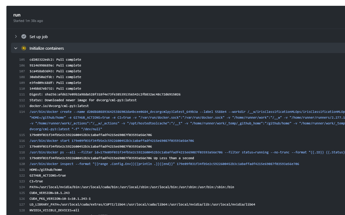
In the details section click on the run itself and the logs can be reviewed in real time. First GitHub is acquiring a container image to install the necessary python configuration to run the train_pipeline.py script. action detail 1

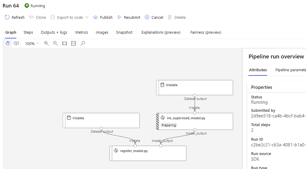
Once the image is acquired, it kicks off the Azure ML Pipeline which can be reviewed in Azure ML Studio action pipeline

pipeline_run1.wait_for_completion() is an important line in train_pipeline.py that keeps the script from completing until the Azure ML pipeline completes. Without this line the action will finish while the pipeline is still running. This may be desired depending on the scenario.

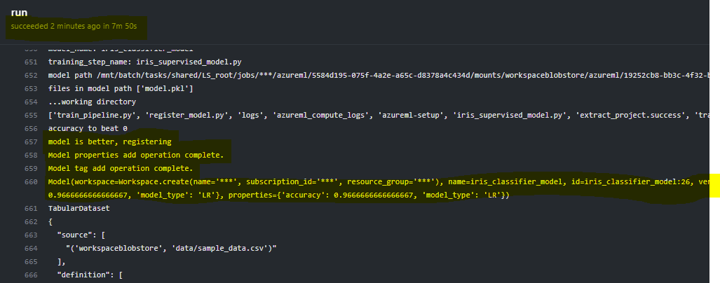
The logged pipeline outputs will be displayed in the run output. action complete logs

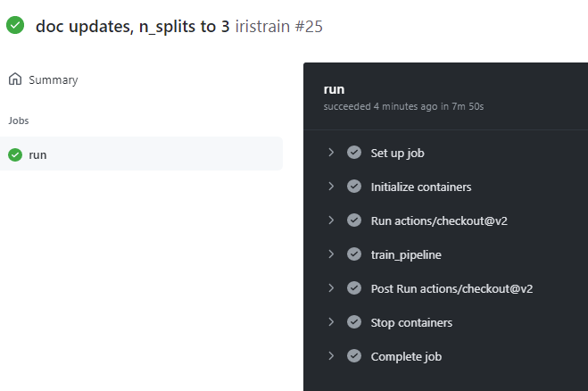
When it is complete, the status will show green. acton complete

Conclusion

That is it. Now your training process is fully automated based on code check in. And yes, YAML is still the most awful definition language but you have to just shut up and deal with it 🙂

Azure ML Pipelines and MLOps with GitHub Actions – Part 2

It is usually better to start at the beginning so you might want to head over to Part 1 if you missed it.

In Part 2 I will focus on managing the pipeline run with the “run context” and then registering the model in a way that ties the model back to the pipeline, artifacts, and code that published it. In Part 3 I will conclude with pipeline schedules and GitHub Actions.

All of the source code can be found on my GitHub so don’t be shy to give it a star 🙂

Leveraging Run Context

Azure ML allows execution of a Python script in a container that can be sent/run on AML compute clusters instead of a local machine. This could be a data transformation script, a training script, or an inferencing script. The below examples shows how to do this for a simple training script (stand alone, in absence of a pipeline)

from azureml.core import Experiment
experiment_name = 'train-on-amlcompute'
experiment = Experiment(workspace = ws, name = experiment_name)

from azureml.core import ScriptRunConfig
src = ScriptRunConfig(source_directory=project_folder, 
                      script='train.py', 
                      compute_target=cpu_cluster, 
                      environment=myenv)
 
run = experiment.submit(config=src)

These "runs" are executed via a submit command from an experiment. Being able to log information to the run from within the script itself (in the above example train.py) is key.

In this repo, iris_supervised_model.py leverages run context to log metrics, tables, and properties. run = Run.get_context() This is the magic line that connects a vanilla Python script to the context of the run, inside the experiment, inside the Azure ML workspace.

Now, metrics can be logged
run.log("accuracy",best_score)
and tables
run.log_confusion_matrix('Confusion matrix '+name, confusion_matrix(Y_train, model.predict(X_train)))

See this sample notebook for all the things logging.

TIP When relying on run context of Azure ML (such as environment variables being passed in from the driver script) performing the following check early in the script can allow defaults to be set for anything that would have been passed in. This allows for local testing which is a time saver.

if (run.id.startswith('OfflineRun')):
	os.environ['AZUREML_DATAREFERENCE_irisdata'] = '.\sample_data.csv'
	os.environ['AZUREML_DATAREFERENCE_model_output'] = '.\model_output'

Managing the pipeline execution

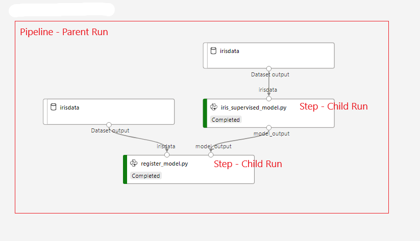
In a pipeline, each run is at the step level, or a child of a parent run which is the pipeline itself.

Pipeline Parent Child

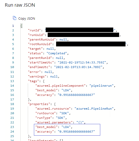
It may be best to log important metrics or properties at the pipeline level rather than at the step level (or both). run.parent will get the parent run context. The code below sets the two properties by passing in a dictionary as the parameter and those same values on two tags as well.

run.parent.add_properties({'best_model':best_model[0],'accuracy':best_score})
run.parent.tag("best_model",best_model[0])
run.parent.tag("accuracy",best_score)

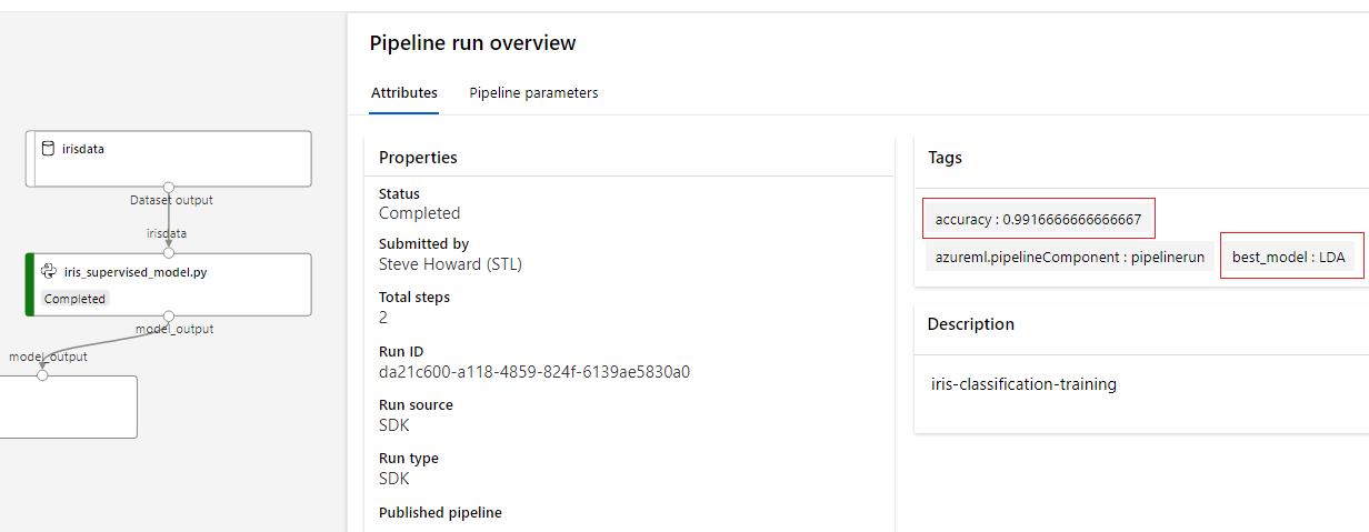
Properties are immutable while tags are not, however tags are more predominant in the Azure ML Run UI so they are easier to read. tags

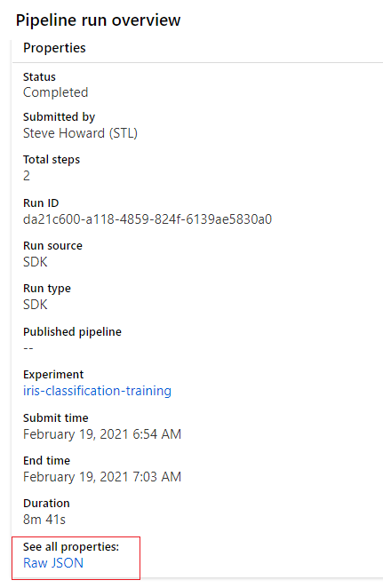
To review the added properties click "Raw JSON" under "see all properties".
see all properties

properties

Now that the results of the training are published to the parent pipeline tags (and properties), they can be used to control what happens in execution of later steps. In register_model.py, the accuracy score is going to control if this model will be registered or not.

Model Registration

The model artifact should be registered as it allows "one click" deployment for real time inferencing hosted on AKS or ACI. Even if the intention is to use it for batch inferencing with Azure ML pipelines it is a more organized way as shown below to keep full context of how the model was built verse just storing the pickle file off in a cloud storage location.

In context of this example pipeline, training has been completed in iris_supervised_model.py. The best model accuracy has been recorded in the tags of the pipeline run.

In the next step of the pipeline register_model.py, retrieve the parent pipeline run context with parentrun = run.parent and review the tags that have been set.

The below code block shows getting the accuracy score from the tag dictionary for the current pipeline run, but also an alternative method to interegate previous steps in the pipeline to retrieve the tags by using parentrun.get_children()

tagsdict = parentrun.get_tags()
if (tagsdict.get("best_model")) != None:
    model_type = tagsdict['best_model']
    model_accuracy = float(tagsdict['accuracy'])
    training_run_id = parentrun.id
else:
    for step in parentrun.get_children():
        print("Outputs of step " + step.name)
        if step.name == training_step_name:
                tagsdict = step.get_tags()
                model_type = tagsdict['best_model']
                model_accuracy = float(tagsdict['accuracy'])
                training_run_id = step.id

The model can be registered directly to the workspace, but the context of how the model was built is then disconnected from the training pipeline. Instead, the model will be registered from the pipeline run object. To do this the model artifact (model.pkl file) needs to be uploaded to the parent run.

# to register a model to a run, the file has to be uploaded to that run first.
model_output = os.environ['AZUREML_DATAREFERENCE_model_output']
parentrun.upload_file('model.pkl',model_output+'/model.pkl')

Next, see if the model name is already registered. If so, record the accuracy score of the previous model to compare against the new model. If this is the first time the model has been trained it won’t exist in the registry so set the accuracy to beat equal to 0.

try:
    model = Model(ws, model_name)
    acc_to_beat = float(model.properties["accuracy"])
except:
    acc_to_beat = 0

Compare the new model accuracy with the previous model accuracy to beat and if the model is better, register it. Note: the model is being registered via parentrun.register_model and not Model.register_model. This is important as it nicely ties the registered model and artifact back to all the context of how it was created.

if model_accuracy > acc_to_beat:
    print("model is better, registering")

    # Registering the model to the parent run (the pipeline). The entire pipeline encapsulates the training process.
    model = parentrun.register_model(
                       model_name=model_name,
                       model_path=model_path,
                       model_framework=Model.Framework.SCIKITLEARN, 
                       model_framework_version=sklearn.__version__,
                       sample_input_dataset=dataset,
                       resource_configuration=ResourceConfiguration(cpu=1, memory_in_gb=0.5),
                       description='basic iris classification',
                       tags={'quality': 'good', 'type': 'classification'})

Set additional properties for accuracy and model_type so that the next time training is ran the current accuracy will be compared against that model (just like above)

model.add_properties({"accuracy":model_accuracy,"model_type":model_type})
model.add_tags({"accuracy":model_accuracy,"model_type":model_type})

Access the run logs, outputs, code snapshots from registered model

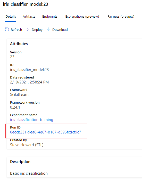
In the model registry, when registering from the run itself, it hyperlinks to the run id.
Model

This links back to the pipeline run.
Pipeline

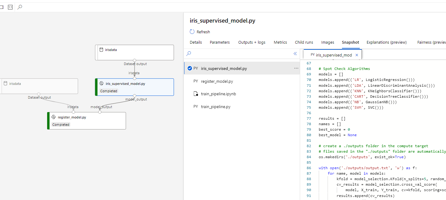
Notice that when clicking on the iris_supervised_model.py step, there is access to the outputs/logs, metrics, and even the snapshots of the code used to generate the model artifact that is registered.
Snapshot

Conclusion

Registering the model from the pipeline run gives complete context of how the model was built and registered! Its sets up real time and batch inferencing deployment as next steps.

Up Next Part 3

Azure ML Pipelines and MLOps with GitHub Actions – Part 1

I have been working on customer projects with Azure ML pretty regularly over the last two years. Some common challenges:

  • Microsoft highly promotes the AKS deployment for real time inference, yet most of the time customers are still looking for an effective way to do batch scoring.
  • When customers leverage Azure ML pipelines for batch processes they struggle with the concept of pushing datasets and files between steps. This erodes the true power of splitting an ML process into steps.
  • MLOps is hard and overwhelming.

This is not a “start from the beginning” blog post. This is going to assume that you have familiarity with Azure ML If you are not, the sample notebooks are seriously EXCELLENT! However, they seem to get you 90% there but miss out on implementation details that are key for success.

The scenario I am using below and can be found on my GitHub. It is an Azure Pipeline that trains several iris classification models. It picks the best one and logs it. In the next pipeline step, if that model is better than the previous training run, it will register the model. This training pipeline can be put on a schedule or it can be triggered from a code check in. In this case, from a GitHub action.

In a later blog post, i will discuss in more detail the model registration process (some production tips there) and the GitHub action, but I will start with properly passing datasets and files between steps.

Passing datasets and files between steps

Other than a few blogs I have found on the internet, instructions on how to properly pass files or datasets between steps are hard to find.

pipeline_image.PNG

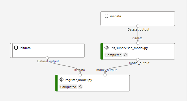
In the above image you can see that irisdata is passed into iris_supervised_model.py and then model_output is the output. When you define the pipeline in the driver script, the input data is a DataReference object and any data passed between steps is a PipelineData object.

from azureml.core.datastore import Datastore
from azureml.data.data_reference import DataReference
ds = ws.get_default_datastore()
print("Default Blobstore's name: {}".format(ds.name))

dataset_ref = DataReference(
    datastore=ds,
    data_reference_name='irisdata',
    path_on_datastore="data/sample_data.csv")
print("DataReference object created")
from azureml.pipeline.core import Pipeline, PipelineData
model_output = PipelineData("model_output",datastore=ds)
print("PipelineData object created for models")

In the PythonScriptStep, utilize the input and output parameters.

from azureml.pipeline.steps import PythonScriptStep
trainingScript = PythonScriptStep(
    script_name="iris_supervised_model.py", 
    inputs=[dataset_ref],
    outputs=[model_output],
    compute_target=aml_compute, 
    source_directory="./azureml",
    runconfig=run_config
)

Simply pass the “model_output” from outputs as input to the next step (the register_model.py that will be a focus of the next blog post) and so on.

Using these references in the script

When you submit a pipeline job to run, a container is created and all the files in the source_directory specified in the PythonScriptStep are imported into the container. The input and outputs effectively become mount points for blob storage to that container. In the iris_supervised_model.py script step this mount point is accessible via an environment variable that looks like the below.

os.environ['AZUREML_DATAREFERENCE_irisdata']

This is also the same environment variable format used for the output location (the PipelineData object) which appears to be a randomly created storage location given to you from AzureML.

mounted_output_path = os.environ['AZUREML_DATAREFERENCE_model_output']

Looking at the mounted_output_path variable above gives a location like: mnt/batch/tasks/shared/LS_root/jobs/amlworkspacesjh/azureml/715a1dca-fafc-4899-ae78-ffffffffffff/mounts/workspaceblobstore/azureml/71ab64d9-bc4c-4b74-a5a5-ffffffffffff/model_output


You should be able to treat these environment variables as a file location just like a local path. So for the irisdata which was a csv file in the data reference you can read it like normal.

df = pd.read_csv(os.environ['AZUREML_DATAREFERENCE_irisdata'], names=column_headers)

For the model_output we pickle the model file and save it to the mounted_output_path.

pkl_filename = "model.pkl"
mounted_output_path = os.environ['AZUREML_DATAREFERENCE_model_output']
with open(os.path.join(mounted_output_path, pkl_filename), 'wb') as file:
    pickle.dump(best_model[1], file)

Now look into register_model.py, we utilize the PipelineData object (model_output) as our input and reference the same environment variable as in iris_supervised_model.py

mounted_output_path = os.environ['AZUREML_DATAREFERENCE_model_output']
print("model path",model_output)
print("files in model path",os.listdir(path=model_output))

In the file list, model.pkl is there right where it was created in the training script.

Conclusion

The ability to pass data between pipeline steps is pretty easy, but the documentation on using the magic “AZUREML_DATAREFERENCE_***” environment variables is lacking in most of the sample notebooks I have found. Just remember that these are mount points and can be interacted with just like local files basically.

Up next, Part 2

The “where have I been?” footnote

It has been 21 months since my last blog post. My role at Microsoft has led me to focus much more on cloud data services for only a couple of customers. I loved to blog about Power BI but I just haven’t been in that space for awhile as my day to day responsibilities were handed over to the much more capable @notaboutthecell. I have been working a lot on real time stream processing (with Databricks / Cosmos DB / Azure Functions) and ML engineering activities with Azure ML. Blog posts have been difficult as so much of my work is implementation oriented and it is hard to recreate everything in a publicly sharable way.

Or maybe i have just been lazy 🙂

Anyway, I am sure that the blog posts in my future are probably going to be more narrow in application and probably won’t be “marathon reads” that explain everything in detail but hopefully enough to connect the dots for the people who need it.

Regular Expressions will save your life!

I am closing out 2017 with a refreshing project that has led me away from Power BI for a bit. However, even for the Power BI community, I think the below information is valuable because at some point, you are going to run into a file that even the M language (Power BI Query Editor) is going to really have a hard time parsing.

For many of you, its still a flat file world where much of your data is being dropped via an FTP server and then you have a process that parses it and puts it in your data store. I recently was working with a file format that I have no idea why someone thought it was a good idea, but nonetheless, i am forced to parse the data. It looks like this:

display > e1
Site Name   : Chicago IL                  Seq Number     : 111
Mile Mrkr   : 304.40                      DB Index #     : 171

Direction   : South                       Arrival        : 00:02  09-22-2017
Speed In/Out: 33/18 MPH                   Departure      : 00:03:45
Slow Speed  : 38 MPH                      Approach Speed : 0 MPH
                                          Approach Length: ~0.0 Feet

Amb Temp    : 81 F                        Battery Voltage: 12.03

Axles       : 5                           Truck Length   : 56.0 Feet
Alarms      : 0                           Cars           : 1
Integ Fails : 0                           Gate A Cnt     : 1
System Warn : 0                           Gate B Cnt     : 1
Weight      : 72000
HBD Filter  : 13 Point Median Filter
Car   Axle   Weight   Ch1   Ch2
Num    Num   (LBS)    (F)   (F)   Alarms
-------------------------------------------------------------- Weight Units = LBS
  1      1    17000.0   N/A   N/A
         2    17000.0   N/A   N/A
         3    17000.0   N/A   N/A
         4    17000.0     0     0
         5    17000.0     0     0

This data simulates truck weigh-in station data. There is a lot of “header” information followed by some “line” items.

Just think for a moment how you would approach parsing this data? Even in Power BI, this would be extremely brittle if we are counting spaces and making assumptions on field names.

What if a system upgrade effecting the fields in the file is rolled out to the truck weigh stations over the course of several months? Slight changes to format, spacing, field names, etc… could all break your process.

 Regex to the Rescue

In my career as a developer, I never bothered to understand the value of regular expressions (regex). With this formatted file I now see that they can save my life (well, that may be dramatic, but they can at least save me from a very brittle pre-processing implementation)

For anyone unfamiliar with regex, a regular expression is simply a special text string for describing a search pattern. The problem is, they are extremely cryptic and scary looking and you want to immediately run away from them and find a more understandable way to solve your text string problem. For instance, a regular expression that would find a number (integer or decimal) in a long string of characters would be defined as

d+(.d*)?

What the heck is that?

The “d” represents any decimal digit in Unicode character category [Nd]. If you are only dealing with ASCII characters “[0-9]” would be the same thing. The “+” represents at least one instance of this pattern followed by (.d*) which identifies an explicit dot “.” followed by another d but this time with a “*” indicating that 0 to n instances of this section of the pattern unlike the first section that required at least 1 instance of a digit. Therefore this should result in true for both 18 as well as 18.12345. However, regex are greedy by default, meaning it expects the full pattern to be matched. So without adding the “?” to the end of the string, the above regex would NOT recognize 18 as a number. It would expect a decimal of some sort. Because we have included the “?” it will end the match pattern as long as the first part of the match was satisfied, therefore making 18 a valid number.

So, the regex was 11 characters and it took me a large paragraph to explain what is was doing. This is why they are under utilized for string processing. But if you are looking at it the other way, it only took 11 characters to represent this very descriptive pattern. Way cool in my book!

Regex language consistency

My example above was from Python. As i am a “data guy”, i find Python to have the most potential for meeting my needs. I grew up on C# and Java however so understanding regex may have some slight variations between languages. Some interesting links on this are below:

Stack Overflow: https://stackoverflow.com/questions/12739633/regex-standards-across-languages

language comparison on Wikipedia: https://en.wikipedia.org/wiki/Comparison_of_regular_expression_engines

Building a Parser using Regex

This file has all kinds of problems. Notice the value formats below:

Temperature: 81 F
Length: 56 Feet
Datetime: 00:02 09-22-2017
Time: 00:03:45
Speed: 33/18 MPH

In addition to text and numeric values, we also have to deal with these additional formats that should be treated as either numeric or datetime values.

I am going to use Python to parse this file and will use a “tokenizer” pattern discussed in the core Python documentation for the re (regex) library: https://docs.python.org/3.4/library/re.html

This pattern will allow us to assign a “type” to each pattern that is matched so we do not have to count spaces and try to look for explicitly named values which could break with any slight modifications to the file.

Below is a function that returns a named tuple with values for the type, the value, the line, and the column it was found in the string.

import re
import collections

Token = collections.namedtuple('Token', ['typ', 'value', 'line', 'column'])

def tokenize(line):
    token_specification = [
        ('SPEED_IN_OUT',    r'(d+(.d*)?/d+(.d*)?s{1}MPH)'),  # speed with multiple values (ex. 15/10 MPH)
        ('SPEED',           r'(d+(.d*)?s{1}MPH)'),  # speed with one value (ex. 10 MPH)
        ('LENGTH',          r'(d+(.d*)?s{1}Feet)'),  # length in feet (ex. 10 Feet)
        ('TEMP',            r'(d+(.d*)?s{1}[F])'),  # Temperature in Fahrenheit (ex. 83 F)
        ('DATETIME',        r'(d+:(d+(:d)*)*)+s+(d+-d+-d+)'),  # Datetime value (ex. 00:00:00  12-12-2017)
        ('TIME',            r'(d+:(d+(:d)*)*)+'),  # time value only (ex. 00:02   or   ex.  00:02:02)  
        ('ID_W_NBR',        r'(d+(.d*)?s([/w]+s?)+)'),  # ID that is prefixed by a number    
        ('NUMBER',  r'd+(.d*)?'),  # Integer or decimal number    
        ('ID',      r'([/w]+s?)+'), # Identifiers
        ('ASSIGN',  r': '),           # Assignment operator
        ('NEWLINE', r'n'),           # Line endings
        ('SKIP',    r'[ t]+'),       # Skip over spaces and tabs
    ]
    tok_regex = '|'.join('(?P<%s>%s)' % pair for pair in token_specification)

    line_num = 1
    line_start = 0
    for match in re.finditer(tok_regex, line):
        kind = match.lastgroup
        value = match.group(kind)
        if kind == 'NEWLINE':
            line_start = match.end()
            line_num += 1
        elif kind == 'SKIP':
            pass
        else:
            column = match.start() - line_start
            token = Token(kind, value.strip(), line_num, column)
            yield token

In my list of token specifications, i have included the most restrictive matches first. This is so that my value for “56.0 Feet” won’t be mistaken for “56.0 F” which would have it identified as a TEMP instead of LENGTH. (I should also be accounting for Celsius and Meters too but i am being lazy)

Let’s look a bit closer at a couple more of these regex.

        (‘ASSIGN’r‘: ‘),           # Assignment operator

The assign operator is very important as we are going to use each instance of this to identify a rule that the NEXT token value should be ASSIGNED to the previous token value. The “little r” before the string means a “raw string literal”. Regex are heavy with “” characters, using this notation avoids having to do an escape character for everyone of them.

        (‘DATETIME’,        r(d+:(d+(:d)*)*)+s+(d+-d+-d+)),  # Datetime value (ex. 00:00:00  12-12-2017)

Datetime is taking the numeric pattern I explained in detail above but slightly changing the “.” to a “:”. In my file, i want both 00:00 and 00:00:00 to match the time portion of the pattern, so therefore I use a nested “*” (remember that means 0 to n occurrences). The + at the end of the first section means at least 1 occurrence of the time portion, therefore simply a date field will not match this datetime regex. Then the “s” represents single or multiple line spaces (remember that regex is greedy and will keep taking spaces unless ended with “?”). Then the last section for the date will take any integer values with two dashes (“-“) in between. This means 2017-01-01 or 01-01-2017 or even 2017-2017-2017 would match the Datetime date section. This may be something I should clean up later 🙂

    tok_regex = ‘|’.join(‘(?P<%s>%s)’ % pair for pair in token_specification)


I wanted to just quickly point out how cool it is that Python then allows you to take the list of regex specifications and separate them with a “|” by doing the “|”.join() notation. This will result in the crazy looking regex below:

‘(?P<SPEED_IN_OUT>(\d+(\.\d*)?/\d+(\.\d*)?\s{1}MPH))|(?P<SPEED>(\d+(\.\d*)?\s{1}MPH))|(?P<LENGTH>(\d+(\.\d*)?\s{1}Feet))|(?P<TEMP>(\d+(\.\d*)?\s{1}[F]))|(?P<DATETIME>(\d+:(\d+(:\d)*)*)+\s+(\d+-\d+-\d+))|(?P<TIME>(\d+:(\d+(:\d)*)*)+)|(?P<ID_W_NBR>(\d+(\.\d*)?\s([/\w]+\s?)+))|(?P<NUMBER>\d+(\.\d*)?)|(?P<ID>([/\w]+\s?)+)|(?P<ASSIGN>: )|(?P<NEWLINE>\n)|(?P<SKIP>[ \t]+)’

Two important things were done here. We gave each specification the ?P<name> notation which allows us to reference a match group by name later in our code. Also, each token specification was wrapped with parenthesis and separated with “|”. The bar is like an OR operator and evaluates the regex from left to right to determine match, this is why i wanted to put the most restrictive patterns first in my list.

The rest of the code iterates through the line (or string) that was given to find matches in using the tok_regex expression and yields the token value that includes the kind (or type) of the match found and the value (represented as value.strip() to remove the whitespaces from beginning and end).

Evaluating the Output

Now that our parser is defined, lets process the formatted file above. We add some conditional logic to skip the first line and any lines that have a length of zero. We also stop processing whenever we no longer encounter lines with “:”. This effectively is processing all headers and we will save the line processing for another task.

lines = list(csv.reader(open('truck01.txt',mode='r'),delimiter='t'))

counter = 0
ls = []
for l in lines:

    if len(l)==0 or counter == 0:
        counter += 1
        continue

    str = l[0]
    index = str.find(":")
    if(index == -1 and counter != 0):
        break

    print(str)
    for tok in tokenize(l[0]):
        print(tok)

    counter += 1

The first few lines processed will result in the following output from the print statements (first the line, then each token in that line)

Site Name   : Chicago IL                  Seq Number     : 111
Token(typ=’ID’, value=’Site Name’, line=1, column=0)
Token(typ=’ASSIGN’, value=’:’, line=1, column=12)
Token(typ=’ID’, value=’Chicago IL’, line=1, column=14)
Token(typ=’ID’, value=’Seq Number’, line=1, column=42)
Token(typ=’ASSIGN’, value=’:’, line=1, column=57)
Token(typ=’NUMBER’, value=’111′, line=1, column=59)
Mile Mrkr   : 304.40                      DB Index #     : 171
Token(typ=’ID’, value=’Mile Mrkr’, line=1, column=0)
Token(typ=’ASSIGN’, value=’:’, line=1, column=12)
Token(typ=’NUMBER’, value=’304.40′, line=1, column=14)
Token(typ=’ID’, value=’DB Index’, line=1, column=42)
Token(typ=’ASSIGN’, value=’:’, line=1, column=57)
Token(typ=’NUMBER’, value=’171′, line=1, column=59)
Direction   : South                       Arrival        : 00:02  09-22-2017
Token(typ=’ID’, value=’Direction’, line=1, column=0)
Token(typ=’ASSIGN’, value=’:’, line=1, column=12)
Token(typ=’ID’, value=’South’, line=1, column=14)
Token(typ=’ID’, value=’Arrival’, line=1, column=42)
Token(typ=’ASSIGN’, value=’:’, line=1, column=57)
Token(typ=’DATETIME’, value=’00:02  09-22-2017′, line=1, column=59)
Speed In/Out: 33/18 MPH                   Departure      : 00:03:45
Token(typ=’ID’, value=’Speed In/Out’, line=1, column=0)
Token(typ=’ASSIGN’, value=’:’, line=1, column=12)
Token(typ=’SPEED_IN_OUT’, value=’33/18 MPH’, line=1, column=14)
Token(typ=’ID’, value=’Departure’, line=1, column=42)
Token(typ=’ASSIGN’, value=’:’, line=1, column=57)
Token(typ=’TIME’, value=’00:03:45′, line=1, column=59)
Slow Speed  : 38 MPH                      Approach Speed : 0 MPH
Token(typ=’ID’, value=’Slow Speed’, line=1, column=0)
Token(typ=’ASSIGN’, value=’:’, line=1, column=12)
Token(typ=’SPEED’, value=’38 MPH’, line=1, column=14)
Token(typ=’ID’, value=’Approach Speed’, line=1, column=42)
Token(typ=’ASSIGN’, value=’:’, line=1, column=57)
Token(typ=’SPEED’, value=’0 MPH’, line=1, column=59)
Approach Length: ~0.0 Feet
Token(typ=’ID’, value=’Approach Length’, line=1, column=42)
Token(typ=’ASSIGN’, value=’:’, line=1, column=57)
Token(typ=’LENGTH’, value=’0.0 Feet’, line=1, column=60)

Notice how everything is being parsed beautifully without having to do any counting of spaces or finding explicit header names. With being able to identify “SPEED”, “TIME”, “LENGTH”, we will also be able to write a function to change these to the proper type format and add a unit of measure column if needed.

The only assumptions we are going to make to process this header information are as below:

1. skip the first line
2. end processing when a non-empty line no longer has an assignment operator of “:”
3. pattern expected for each line is 0 to n occurrences of ID ASSIGN any_type

To handle #3 above, we add the below code to the end of the for loop shown above:

    dict = {}
    id = None
    assign_next_value = False
    for tok in tokenize(l[0]):
        print(tok)
        if tok.typ == "ASSIGN":
            assign_next_value = True
        elif assign_next_value:
            dict = {id:tok.value}
            print(dict)
            ls.append(dict)
            assign_next_value = False
            id = None
            dict = {}
        else:
            id = tok.value

If you follow the logic, we are just taking the string (each line of the file) and recording the value of the first token as the id, finding the assign operator “:”, and then recording the following token value as the value of a dictionary object. It then appends that dictionary to the “ls” list that was initialized in the first code snippet.

We could then format it as JSON by adding the below line of code after the for loop

import json
jsondata = json.dumps(ls,indent=2,seperators=(",",":"))

See output below, some additional formatting work needs to be done with this as well as pre-processing my numbers and date times to not be represented as strings, but that is not the focus of this blog post.

[
  {
    "Site Name":"Chicago IL"
  },
  {
    "Seq Number":"111"
  },
  {
    "Mile Mrkr":"304.40"
  },
  {
    "DB Index":"171"
  },
  {
    "Direction":"South"
  },
  {
    "Arrival":"00:02  09-22-2017"
  },
  {
    "Speed In/Out":"33/18 MPH"
  },
  {
    "Departure":"00:03:45"
  },
  {
    "Slow Speed":"38 MPH"
  },
  {
    "Approach Speed":"0 MPH"
  },
  {
    "Approach Length":"0.0 Feet"
  },
  {
    "Amb Temp":"81 F"
  },
  {
    "Battery Voltage":"12.03"
  },
  {
    "Axles":"5"
  },
  {
    "Truck Length":"56.0 Feet"
  },
  {
    "Alarms":"0"
  },
  {
    "Cars":"1"
  },
  {
    "Integ Fails":"0"
  },
  {
    "Gate A Cnt":"1"
  },
  {
    "System Warn":"0"
  },
  {
    "Gate B Cnt":"1"
  },
  {
    "Weight":"72000"
  },
  {
    "HBD Filter":"13 Point Median Filter"
  }
]

Now What?

I hope to do a continuation of this blog post and explore a server-less architecture of taking the file from the FTP server, immediately running this pre-processing, and dumping the JSON out to a stream ingestion engine. From there, we can do all sorts of cool things like publish real time data directly to Power BI, or into a Big Data store. This follows principles of “Kappa Architecture”, a simplification of “Lambda Architecture” where everything starts from a stream and the batch processing layer goes away.

There are multiple ways to implement this, but with Cloud computing, we have an opportunity to do this entire chain of events in a “server-less” environment meaning no virtual machines or even container scripts have to be maintained. So, lets cover this next time

Conclusion

Regex are super powerful. I ignored them for years and now I feel super smart and clever for finding a better solution to file processing than i would have originally implemented without regex.

The full Python code from above as well as the formatted file can be found on my GitHub here


Working with Scatter Plots in Power BI

I really like some of the advancements that have been made in Power BI scatter plots over the last few months. I wanted to point out some capabilities you may not be using that maybe you should be.

Data Sampling Improvements

In the September 2017 release, you can now be confident that all of your outliers are being shown. No one can visually look at a plot and interpret several thousand data points at once, but you can interpret which of those points may be outliers. I decided to test this out myself between a Python scatter plot of 50k data points and Power BI.

In the test, I used a randomly generated normal distribution of 50k data points to ensure I had some outliers.

#Create a random dataset that has a normal distribution and then sort it (in this case, 50000 data points)
x = np.random.normal(50,25,50000)
x = np.sort(x)

#Create another dataset to put on the y axis of the scatter plot
y = np.random.normal(50,25,50000)

#plot the dataset
plt.scatter(x,y,alpha=0.3)
plt.show()

(You can see the Python notebook on my GitHub here).

Here it is in Python:

Here it is in Power BI (September desktop release)

Notice that all the outliers have been preserved. Note that in previous releases, the Power BI rendering of this would have been shown as below.

This is a great improvement. To learn more about this update, check out the official blog post on high density sampling: https://powerbi.microsoft.com/en-us/documentation/powerbi-desktop-high-density-scatter-charts/

Working with Outliers (Grouping)

Now that we know the dense sampling is preserving our outliers, we can perform some analysis on them. Power BI makes it easy to CTRL+click on multiple outliers and then right-click and add new Group

This will create a new field in your fields list for this group of outliers and will automatically include a Group for “Other” (the other 49.993 data points that weren’t selected). Note that I renamed my field to “High Performers”

As this is a random dataset with integers for x,y values there are no dimensions here that may be interesting to compare, but consider now we can always come back to this grouping for further analysis such as the bar chart below:

Clustering

You can also use “…” in the upper right of the scatter chart to automatically detect clusters. Our example again is a bit uninteresting due to it being a random normal distribution but gives you an idea of how you can cluster data that is more meaningful.

Symmetry Shading and Ratio Lines

These gems were released in the August 2017 desktop release and really helps visualize the skew of your data.

Both of these can be turned on from the analytics tab.

Instead of using our sample dataset above I will use the dataset from my last blog post on Scorecards and Heatmaps.

In the below plot I took the SalesAmount field and plotted on the y axis against the SalesAmountQuota field on the x axis. From Symmetry shading we can observe that none of our sales people are meeting their quota. From the ratio line we can see the few individuals that have a positive variance to the ratio while most are flat or below the ratio.

You can read more about these two features in the August Desktop blog post: https://powerbi.microsoft.com/en-us/blog/power-bi-desktop-august-2017-feature-summary/#symmetryShading

Conclusion

These are just a few of the recently released features that I think have made the native scatter chart in Power BI a very useful visual. I have posted the PBIX file for the normal distribution data on my GitHub if you would like to download: https://github.com/realAngryAnalytics/angryanalyticsblog/tree/master/20171002-scatterplots


Deep Learning Toolkit considerations for emerging data scientists

Overview

Disclaimer: This blog is my own opinion and not that of my employer, however it should be noted that I am a Microsoft employee and this may reflect that perspective.

Update: New version of these benchmarks is being worked on and can be tracked here: http://dlbench.comp.hkbu.edu.hk/

This post is a departure from my usual focus on Power BI. Enterprise deployment scenarios for Power BI have been a great subject for me. However, In my day job, I do work on a variety of data platform related subjects. These are my findings on deep learning toolkits and what you should know before getting too deep into them, especially pay attention to my section on Keras

Deep learning is popular for image processing (computer vision, facial recognition, emotion detection), natural language processing (sentiment analysis, translation), and even starting to find its way into areas such as customer churn. Neural networks with many layers are used to increase precision of a prediction as opposed to more statistical type algorithms such as linear regression.

There are several popular open source deep learning toolkits including Caffe, Torch, TensorFlow, CNTK (now Cognitive toolkit), and mxnet

This post will mostly reference TensorFlow and CNTK for reasons established in the section on Keras.

Python vs R

This debate will rage on for probably another decade similar to how I remember the Java vs C# debate as a developer in the early 2000’s. From what I have seen, Python appears to have more support in the area of deep learning than R. All but Torch support Python integration while only TensorFlow and mxnet support R directly.

Toolkit Performance

One of the most important aspects of a deep learning toolkit is performance.

Lets consider a couple of scenarios:

In the software development cycle a poorly indexed table could be the difference in 5 seconds and 5 minutes to call the database. This is annoying but is not the critical path to meeting a deadline. It takes many developer hours and iterations to build the code around that database call making that index issue less significant, but of course something that should be addressed.

In deep learning on the other hand, the difference between a model that performs twice as fast as another toolkit could mean the difference between 1 vs 2 days of training time. The iteration cycle is greatly impacted and retraining a model 5 times could be the difference between 1 week and 2 weeks to deliver results. This is significant!

Benchmarking Performance among leading toolkits

Benchmarking State-of-the-Art Deep Learning Software Tools is an academic journal (latest revision February 2017) comparing the most popular deep learning toolkits for CNN, FCN, and LTSM. These acronyms are neural network types you will want to familiarize yourself with if you are not already. There is a new eDX course that is just starting that you can learn all about these concepts.

Below i have included some links that may be to other frameworks but the content explanations seemed more easily understood

Convolutional Neural Network (CNN) – used primarily for image processing. Popular implementations include:
  • AlexNet – an 8 layer CNN circa 2012 that cut error rate nearly in half from previous versions
  • ResNet-50/101/152/etc – A deep residual learning network with 50/101/152/etc layers respectively circa 2015 achieving an error rate of 3.57% which was 4 times improvement from AlexNet

Fully Convolutional Neural Nework (FCN) – variation of CNN that doesn’t include the fully connected layer

Recurrent Neural Network (RNN) & Long Short Term Memory (LTSM) – widely used for natural language processing

This paper is extremely thorough and as our instincts are to scroll immediately to page 7 to start interpreting the bar charts, it is important to note how they ran these tests and gathered the results as described in pages 1-6.

One summary table that doesn’t fully represent all results is shown below.

Shaohuai Shi, Qiang Wang, Pengfei Xu, Xiaowen Chu, “BenchmarkingState-of-the-ArtDeepLearningSoftwareTool”

As you interpret these results, as well as the rest of them in the journal, you will notice three glaring observations

  • There is not one toolkit that has best performance across all neural network types. In fact, there can be wide variation in performance rank for a single toolkit based on # of CPUs or # of GPUs used.
  • Google TensorFlow is arguably the most popular of all of these toolkits, yet the results published in this paper other than in a few cases show it is quite average if not consistently poorer performing than others.
  • CNTK is orders of magnitude better than all of the competition in LTSM

Note on Google TensorFlow

CNTK performs better overall and by orders of magnitude in some cases to TensorFlow. As emerging data scientists start to pick toolkits for deep learning, TensorFlow seems to be a popular choice. In many cases, it will have desirable performance, but to put “all your eggs in one basket” so to speak, may not be the best approach here.

I actually am a fan of TensorFlow and picking a toolkit on performance alone would also not be wise. TensorFlow has some neat features one being TensorBoard that helps visualize the execution graph (note that CNTK also supports TensorBoard). Google has also recently introduced a dedicated TensorFlow processor (TPU) when running on their cloud platform that will surely speed up processing time. But if you are doing NLP (natural language processing), it is quite obvious you would want to use CNTK for performance reasons…

What is an emerging data scientist to do?

This is where Keras comes in…

Keras

Keras is an abstraction layer that allows you to run the same code on top of both TensorFlow and CNTK (as well as Theano, another deep learning toolkit) as the backend.

For Big Data people, I would make a correlation between Keras and the use of HIVE as an abstraction layer for Map/Reduce. It is rare to actually write Map/Reduce code anymore with the evolution of libraries around big data, and that is what Keras reminds me of compared to actually writing TensorFlow (or CNTK) code. For instance, TensorFlow on its own actually requires you to write the formula for Mean Squared Error to pass into the model. Although trivial, this is totally annoying and the use of Keras builds a lot of shortcuts for us that makes life much easier and reduces code often by 50%.

In the keras.json file that is created during installation, the backend can be configured by changing one line between “tensorflow” and “cntk”

{
    "floatx": "float32",
    "epsilon": 1e-07,
    "backend": "cntk",
    "image_data_format": "channels_last"
}

to verify the backend that is being used, from python simply enter

import backend from keras

or at anytime you can access the _BACKEND variable from the same library to see the result

These details are all described clearly on the keras.io site referenced above.

…and for all of the R users, there is a nice CRAN package available too:
https://cran.r-project.org/web/packages/kerasR/vignettes/introduction.html

from my somewhat limited experience, I can say that using Keras on top of TensorFlow or CNTK keeps me from pulling my hair out. Kudos to the creators and contributors to this library. Maybe we can dive deeper into this in a future post.

Transfer Learning

Transfer learning is the ability to take a preexisting model and use it as the base for another model. This allows you to take for instance a model that has classified millions of images and has trained for possibly weeks and apply it to new images that are more specific to your scenario. This allows for more rapid model development if you can build on preexisting work.

CNTK has a really nice tutorial on this technique here:
https://docs.microsoft.com/en-us/cognitive-toolkit/build-your-own-image-classifier-using-transfer-learning

TensorFlow also has it’s own “Inception” library that can be transferred.

This concept is the basis for the next section of “Deep Learning as a Service”

Deep Learning as a Service

I don’t believe this has actually become a term yet. I am just making it up as I go here 🙂

The concept of transfer learning opens some new capabilities to more easily apply your own scenarios to previously trained models.

Microsoft has developed a few interesting services that make deep learning very accessible to end users

One is the Custom Vision Service: https://www.customvision.ai/

This allows you to bring your own images to train on and allows you to reinforce in an iterative approach

Another is Q&A Maker: https://qnamaker.ai/

this allows you to build a bot in minutes to scroll through FAQ and document content on a subject that is important to your organization. This bot can then interact in an intelligent way without having to use a deep learning toolkit or a bunch of coding.

I did one using the Power BI FAQ pages and it worked really well

What is interesting about these services is that it is actually training a model on YOUR data. Not simply tapping into a pre-existing model. You are able to influence the results.

I believe we will continue to see many more services pop up like this that will continue to “democratize” AI for the masses

Conclusion

I would never claim to be a data scientist, but many of us are doing more and more data science like activities. For a person moving from data and business intelligence into machine learning and artificial intelligence, I feel like the above content would have saved me a lot of time. There is plenty of getting started content out there so start using your google/bing search skills to get deeper into it.